#load packages
library(tidyverse)
library(survival)
library(ggfortify)
library(rstanarm)
library(brms)
library(tidybayes)

theme_set(theme_classic())

Background

I’m working with tree-level data in the Sierra Nevadas centered on root disease gap centers. The trees were originally surveyed in the early 1970s and have been resurveyed every 1-8 years up until post-drought from 2012-2016. I’m interested in running a survival analysis in order to parse the effects of climate and disease on tree mortality. Since basic survival models assume that variables do not change over time, I need to employ a workaround that relaxes that assumption–I’d like to allow climate, DBH and the effects of disease to vary with time.

There seems to be a billion ways and packages to model time-to-events, but one approach is to use a peicewise exponential model, which in effect is similar to the cox proportional hazards model. Essentially, you cut the survival function into smaller intervals, assume the hazard rate is constant within each interval, and independent from the next. Read more about that here, starting on page 17: https://data.princeton.edu/wws509/notes/c7.pdf

A poisson regression is equivalent in form and advantageous since one can model the mean hazard rate the same way as a poisson generalized linear mixed model. The GLMM framework is familiar and affords me the ability to add in additional complexity that canned survival analysis packages cannot.

Here I’m going to show how the poisson model is equivalent by contrasting various models and showing that the coefficients and survival predictions are essentially the same. The models I will contrast are the following:

cox proportional hazard (frequentist)
bayesian survival model with a M-spline and weibull baseline hazard (Rstanarm survival functions)
bayesian poisson trick with and without smoothing term for time (brms)

The last option is the most flexible since you can write a poisson model in any program you’d like. I show it in brms because it’s simple, but for increased flexibility, I’ll eventually write the model for my project in Stan.

The data

Even though I’m interested in using the poisson model because I want to use time-varying covariates, the model can still run fine even when the variables remain constant. For simplicity, that’s what I’ll do.

Let’s work with the leukemia dataset from the package survival.

#leukemia dataset
data(leukemia, package = "survival")

#add an id column
df <- as_tibble(leukemia) %>% 
  mutate(id = seq_len(n())) 
df

## # A tibble: 23 x 4
##     time status x             id
##    <dbl>  <dbl> <fct>      <int>
##  1     9      1 Maintained     1
##  2    13      1 Maintained     2
##  3    13      0 Maintained     3
##  4    18      1 Maintained     4
##  5    23      1 Maintained     5
##  6    28      0 Maintained     6
##  7    31      1 Maintained     7
##  8    34      1 Maintained     8
##  9    45      0 Maintained     9
## 10    48      1 Maintained    10
## # … with 13 more rows

df %>% count(x)

## # A tibble: 2 x 2
##   x                 n
##   <fct>         <int>
## 1 Maintained       11
## 2 Nonmaintained    12

You can see that some patients have a status of 1, meaning they died at the recorded time, while others have a status of 0, meaning they were censored at the recorded time. There’s also a covariate x, which is a binary indicator split equally among the patients.

Here’s what the data look like:

#quick visualization of the data (Kaplan meier)
autoplot(survfit(Surv(time, status)~x, 
        data = df), conf.int = F)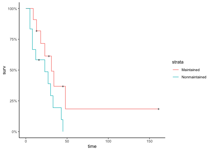

By time=48, everyone except for one person is either dead or has left the study (censored).

Turn data into long format

Currently the data has 1 row per patient. We want 1 row per timepoint-patient. In other words, there will be a row desribing a patient’s status for every time interval that they remained in the study. After a patient dies or is censored, they are no longer in the dataset.

Here, I’ll define the cutpoints by every time there was a death. It’s important that each cutpoint has at least one event, otherwise the model has a difficult time estimating baseline hazards. Then we can use survSplit to aid with making the data long.

#choose cut points
#events only + the last one. 
lasttime <- max(df$time) 
events <- df %>% 
  filter(status == 1) %>% 
  pull(time) %>% unique() %>% sort
cut_events <- c(events, lasttime)

#make long. Want time start/stop, duration, status, covariates. 
df_long <- survSplit(
    formula = Surv(time, status) ~ ., 
    data = df, 
    cut = cut_events) %>%
  rename(tstop = time) %>% 
  mutate(tduration = tstop - tstart)

head(df_long)

##            x id tstart tstop status tduration
## 1 Maintained  1      0     5      0         5
## 2 Maintained  1      5     8      0         3
## 3 Maintained  1      8     9      1         1
## 4 Maintained  2      0     5      0         5
## 5 Maintained  2      5     8      0         3
## 6 Maintained  2      8     9      0         1

Fit with cox proportional hazard model

This is the most basic fit. It’s useful to get an idea of what the covariate estimates should be. The output is identical regardless of whether the data is ‘short’ or long.

fit_cox_short <- coxph(Surv(time, status)~x, 
        data = df)
fit_cox_short #x = 0.92, se=.51

## Call:
## coxph(formula = Surv(time, status) ~ x, data = df)
## 
##                  coef exp(coef) se(coef)     z      p
## xNonmaintained 0.9155    2.4981   0.5119 1.788 0.0737
## 
## Likelihood ratio test=3.38  on 1 df, p=0.06581
## n= 23, number of events= 18

fit_cox_long <- coxph(Surv(tstart, tstop, status)~x, 
        data = df_long)
fit_cox_long #x = 0.92, se=.51

## Call:
## coxph(formula = Surv(tstart, tstop, status) ~ x, data = df_long)
## 
##                  coef exp(coef) se(coef)     z      p
## xNonmaintained 0.9155    2.4981   0.5119 1.788 0.0737
## 
## Likelihood ratio test=3.38  on 1 df, p=0.06581
## n= 180, number of events= 18

Fit with `Rstanarm`

Rstanarm recently came out with new features to model survival data. As of writing this, the functions haven’t been released on CRAN yet but you can download them in the development version from github:
remotes::install_github("stan-dev/rstanarm@feature/survival")
You can learn more here: https://arxiv.org/pdf/2002.09633.pdf

#M-splines (default with default wiggliness arguments)
fit_RSA_ms <- stan_surv(
  Surv(tstart, tstop, status)~x, 
  basehaz = 'ms',
  data = df_long,
  chains = 3, cores = 3, iter = 2000
)
summary(fit_RSA_ms, digits = 2) #x = .89 (.28, 1.53)

## 
## Model Info:
## 
##  function:        stan_surv
##  baseline hazard: M-splines on hazard scale
##  formula:         Surv(tstart, tstop, status) ~ x
##  algorithm:       sampling
##  sample:          3000 (posterior sample size)
##  priors:          see help('prior_summary')
##  observations:    180
##  events:          18 (10%)
##  right censored:  162 (90%)
##  delayed entry:   yes
## 
## Estimates:
##                   mean   sd   10%   50%   90%
## (Intercept)     0.76   0.43 0.21  0.77  1.31 
## xNonmaintained  0.87   0.50 0.23  0.85  1.51 
## m-splines-coef1 0.02   0.02 0.00  0.01  0.04 
## m-splines-coef2 0.06   0.05 0.01  0.05  0.12 
## m-splines-coef3 0.40   0.19 0.15  0.41  0.65 
## m-splines-coef4 0.27   0.19 0.04  0.25  0.55 
## m-splines-coef5 0.13   0.11 0.02  0.10  0.29 
## m-splines-coef6 0.12   0.10 0.01  0.09  0.26 
## 
## MCMC diagnostics
##                 mcse Rhat n_eff
## (Intercept)     0.01 1.00 2289 
## xNonmaintained  0.01 1.00 2631 
## m-splines-coef1 0.00 1.00 3256 
## m-splines-coef2 0.00 1.00 2721 
## m-splines-coef3 0.00 1.00 2256 
## m-splines-coef4 0.00 1.00 2111 
## m-splines-coef5 0.00 1.00 2782 
## m-splines-coef6 0.00 1.00 3343 
## log-posterior   0.06 1.00 1061 
## 
## For each parameter, mcse is Monte Carlo standard error, n_eff is a crude measure of effective sample size, and Rhat is the potential scale reduction factor on split chains (at convergence Rhat=1).

#weibull (a little more familiar, but won't be as similar to coxph)
fit_RSA_w <- update(fit_RSA_ms, basehaz = 'weibull')
summary(fit_RSA_w, digits = 2) #x = 1.14 (.49, 1.81)

## 
## Model Info:
## 
##  function:        stan_surv
##  baseline hazard: weibull
##  formula:         Surv(tstart, tstop, status) ~ x
##  algorithm:       sampling
##  sample:          3000 (posterior sample size)
##  priors:          see help('prior_summary')
##  observations:    180
##  events:          18 (10%)
##  right censored:  162 (90%)
##  delayed entry:   yes
## 
## Estimates:
##                  mean   sd    10%   50%   90%
## (Intercept)    -5.28   1.06 -6.61 -5.18 -4.03
## xNonmaintained  1.20   0.56  0.52  1.17  1.92
## weibull-shape   1.26   0.23  0.99  1.25  1.55
## 
## MCMC diagnostics
##                mcse Rhat n_eff
## (Intercept)    0.04 1.00  878 
## xNonmaintained 0.02 1.00 1033 
## weibull-shape  0.01 1.00  985 
## log-posterior  0.06 1.00  541 
## 
## For each parameter, mcse is Monte Carlo standard error, n_eff is a crude measure of effective sample size, and Rhat is the potential scale reduction factor on split chains (at convergence Rhat=1).

#can easily plot baseline hazard rate
p1 <- plot(fit_RSA_ms)+
  labs(title = 'M-splines baseline haz')
p2 <- plot(fit_RSA_w)+
  labs(title = 'Weibull baseline haz')

#also survival posteriors
ps_ms <- posterior_survfit(fit_RSA_ms, 
                  newdata = data.frame(
                    x = c('Maintained', 'Nonmaintained')),
                  times = 0) %>% 
  mutate(x = ifelse(id == 1, 'Maintained', 'Nonmaintained'))
ps_w <- posterior_survfit(fit_RSA_w, 
                  newdata = data.frame(
                    x = c('Maintained', 'Nonmaintained')),
                  times = 0) %>% 
  mutate(x = ifelse(id == 1, 'Maintained', 'Nonmaintained'))

p3 <- ggplot(ps_ms, aes(time, median, group = x)) +
  geom_line(aes(color = x)) +
  geom_ribbon(aes(ymin = ci_lb, ymax = ci_ub, fill = x), alpha = .4) + theme(legend.position = 'none') +
  labs(title = 'M-splines Survival')
p4 <- ggplot(ps_w, aes(time, median, group = x)) +
  geom_line(aes(color = x)) +
  geom_ribbon(aes(ymin = ci_lb, ymax = ci_ub, fill = x), alpha = .4) + 
  theme(legend.position = 'bottom')+
  labs(title = 'Weibull Survival')

#plot all together
p5 <- cowplot::plot_grid(p1,p2,p3,p4 +theme(legend.position = 'none'))
cowplot::plot_grid(p5, cowplot::get_legend(p4), nrow = 2, rel_heights = c(.9, .1))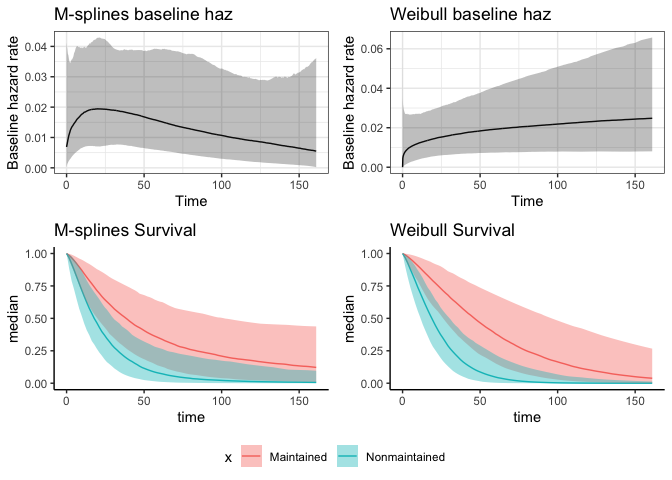

The estimate of the treatment coefficient in the M-splines model was closer to the cox PH model from before because it’s more flexible than the weibull baseline hazard rate.

Clearly this looks like an awesome new set of features, complete with really easy functions to plot the posterior predictions. It’s still a bit too rigid for my needs though since in my project, I’d like to allow the effect of disease to decay in space and time. If you just have linear effects, this seems like a really promising tool!

Poisson trick

Here we’ll use a peicewise exponential model and approximate it with a poisson model. Within each time interval (j), the hazard for individual (i) is defined as

[{ij} = {j} (x^T_i )]

Through some mathematical rearrangement, the hazard can be modeled with a poisson regression. I can’t do the explanation justice, so I’ll just refer readers to this link here. The status of each individual is modeled with a poisson likelihood and the general equation of the mean is

[{ij} = t{ij}_{ij} ]

where (t_{ij}) is the exposure time and (_{ij}) is the hazard rate for individual (i) in interval (j). By logging both sides, we find a familiar poisson equation:

[ log({ij}) = log(t{ij}) + _{j} + x^T_i ]

where (log(t_{ij})) acts as an offset to control for variation in time interval durations, ({j} = log({j})) is the baseline hazard, and (x^T_i ) is where you estimate your covariates. Even though we’re following the same individuals through time, we don’t need an individual-level random intercept because we’re computing each hazard independently. From here, the model can be as complex as you can make any GLMM!

Models in `brms`

Traditionally (_j) is treated as a factor since it’s the intercept for each time interval. You can also use a spline smoother to estimate the baseline hazard as a continuous function. I’ll demostrate both below.

#a_j is a factor
fit_BRM_factor <- brm(
  formula = status ~ as.factor(tstop) + x + offset(log(tduration)),
  family = poisson(),
  prior = set_prior('normal(0, 4)', class = 'b'), 
  data = df_long, chains = 3, cores = 3, iter = 2000)

#a_j is a smooth function that changes over time
#number of knots will be length of cutpoints
fit_BRM_spline <- brm(
  formula = status ~ s(tstop, k = length(cut_events)) + x + offset(log(tduration)),
  family = poisson(),
  prior = set_prior('normal(0, 4)', class = 'b'), 
  data = df_long, chains = 3, cores = 3, iter = 2000)

#increasing delta due to divergent transitions, which kinda helps, but still quite a few DTs. Rhats and neff good, so it converged ok.
fit_BRM_spline <- update(fit_BRM_spline, control = list(adapt_delta = .99))

Let’s now plot the baseline hazard rate for both of these models. It seems like one advantage to applying a smoothing spline for each time interval is so that you can have a continuous hazard rate.

The intercepts represent the log-baseline hazard. We need to get the posterior predictions and exponentiate them to get them on the correct scale.

#baseline hazard, time = factor
haz_timefactor <- tidy_draws(fit_BRM_factor) %>% 
  select(b_Intercept:b_as.factortstop161) %>% 
  mutate_at(vars(contains('as.factor')), .funs = function(x) x + .$b_Intercept) %>% 
  mutate(draw = seq_len(n())) %>% 
  rename(b_as.factortstop5 = b_Intercept) %>% 
  pivot_longer(contains('b_as.factor'), names_prefix = 'b_as.factortstop') %>% 
  mutate(time = as.integer(name))

#plot for time = factor
ggplot(haz_timefactor, aes(as.factor(time), exp(value))) +
  geom_jitter(width = .1, height = 0, alpha = .01) +
  #geom_boxplot() +
  theme(axis.text.x = element_text(angle = 90)) +
  labs(title = 'Hazard for time = factor',
       x = 'time interval (j)', 
       y = expression(paste('baseline hazard (', lambda['j'], ')') ))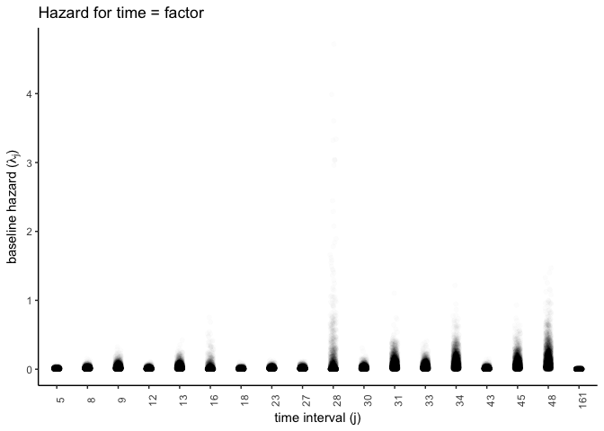

I’ll do the same for the smoothed time function. For some reason knitting with Rmarkdown renders something incorrect, but it works when I run it unknitted. I don’t show the figures, but the code should work.

#do for time = spline function
#predict to new data. Just want the intercept, so x = Maintained, which the model treated as 0 (dummy variable).
newdat <- expand_grid(tstop = 0:lasttime, tduration = 1,
  x = c('Maintained'))
postmu <- fitted_draws(fit_BRM_spline, newdata = newdat, scale = 'linear') #values are log baseline hazard

#estimate median hazard
median_haz <- postmu %>% 
  group_by(tstop) %>% 
  summarise(median_haz = mean(exp(.value)))

#plot hazard for the first 200 draws
postmu %>% filter(.draw %in% 1:200) %>% 
  ggplot(., aes(tstop, exp(.value))) +
  geom_line(alpha = .1, aes(group = .draw))+
  geom_line(data = median_haz, aes(tstop, median_haz), color = 'maroon') +
  scale_y_continuous(limits = c(0, 1.5)) +
  labs(title = 'Hazard for time = spline',
       x = 'time interval (j)', 
       y = expression(paste('baseline hazard (', lambda['j'], ')') ))

It looks like the model is really unsure about the hazard rate after time=50. There’s no event after this time point, so that’s probably why it’s unsure? Let’s plot pre time=50 to see if its similar the one where time is a factor.

#time=spline, time < 50
postmu %>% filter(.draw %in% 1:200, tstop < 50) %>% 
  ggplot(., aes(tstop, exp(.value))) +
  geom_line(alpha = .1, aes(group = .draw))+
  geom_line(data = filter(median_haz, tstop < 50), aes(tstop, median_haz), color = 'maroon', lwd = 1) +
  labs(title = 'Hazard for time = spline, time < 50',
       x = 'time interval (j)', 
       y = expression(paste('baseline hazard (', lambda['j'], ')') ))

I’m not convinced that it’s worth smoothing out the baseline hazard. Already has sampling issues with such a simple dataset and coding in splines is yet another obstacle if I wanted to write this model in Stan.

Compare models

The data has now been fit using 3 different packages, each with slightly different assumptions. Let’s compare the coeffients for the treatment, baseline hazards, and the survival curves.

First, coeffients for the treatment

#extract estimates mean and 90% CI
CIs <- confint(fit_cox_long, parm = 'xNonmaintained', level = .9)
x_coxph <- data.frame(mean = coef(fit_cox_long), 
                      lower = CIs[1], upper = CIs[2]) 

#get posteriors for the rstanarm and brms models
mods <- list(fit_RSA_ms, fit_RSA_w, fit_BRM_factor, fit_BRM_spline)
posts <- lapply(mods, tidy_draws)

#extract treatment coef
f_coef <- function(post){
  whichcol <- grep('maintained', names(post))
  x <- pull(post[,whichcol])
  data.frame(mean = mean(x), lower = hdci(x, .width = .9)[1], upper = hdci(x, .width = .9)[2])
}

trt_coefs <- lapply(posts, f_coef) %>% 
  bind_rows() %>% 
  bind_rows(x_coxph) %>% 
  mutate(model = c('rstanarm m-splines', 'rstanarm weibull', 'brms time factor', 'brms time spline', 'coxph'))
  
ggplot(trt_coefs, aes(mean, model)) +
  geom_pointrange(aes(xmin = lower, xmax = upper)) + 
  scale_x_continuous(limits = c(-1,2.1)) + 
  labs(x = 'treatment coef')

## Warning: Removed 1 rows containing missing values (geom_segment).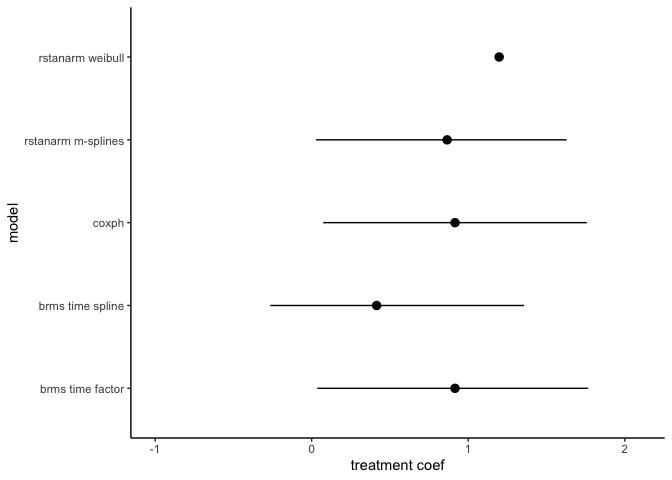

All the estimates are pretty similar. That’s reasurring.

Secondly, survivial curves

Let’s look at the survival curve predictions against observed data. As of now I can’t get posterior predictions with the rstanarm models with tidybayes (major mark against these features until that’s worked out), so I’ll rely on the built-in plotting functions. I will estimate the survival probabilities for the poisson models.

The output of the posterior is the log-hazard rate. The survival function is directly related to the hazard rate:

[S(t) = (-^t_0 (z)dz)] Since our chunks of time are discrete, we add up the cumulative hazards, correct for the exposure time (time between intervals, i.e. the offset), and take the negative exponential:

[ S(t|x)= (-_j (j + log(t{j}) + x)) ] tidybayes::fitted_draws() makes this easy by predicting the mean posterior to new data and already takes into account the exposure time and covariates.

#generate curve for observed data using Kaplan-Meier
surv_obs = fortify(survfit(Surv(time, status)~x, 
                            data = df)) %>% 
  select(tstart=time, surv, x = strata) %>% 
  add_case(tstart = 0, surv = 1, x = c('Maintained', 'Nonmaintained'))


#get posterior predictions from the brms models for both treatments. 

#need to define new dataframe to predict to.
newdat_factor <- data.frame(
  tstart = unique(df_long$tstart),
  tduration = diff(c(0, cut_events)) ) %>% 
  expand_grid(x = c('Maintained', 'Nonmaintained')) %>% 
  mutate(tstop = tstart + tduration)
newdat_spline <- expand_grid(tstop = 0:lasttime, tduration = 1,
  x = c('Maintained', 'Nonmaintained'))


#predict posterior means. automatically adds in the offset when it predicts the posterior. 
PP_factor <- fitted_draws(fit_BRM_factor, newdata = newdat_factor, scale = 'linear') 


#put posterior into nice dataframe for plotting
#factor
surv_factor <- PP_factor %>% 
  #filter(.draw == 1, x=='Maintained') %>% 
  select(-.chain, -.iteration) %>% 
  group_by(.draw, x) %>% 
  mutate(S = exp(-cumsum(exp(.value)))) 
surv_factor_mean <- surv_factor %>% 
  group_by(x, tstop) %>% 
  summarise(S = mean(S))

#spline predictions. I'm commenting this out since it doesn't knit properly.
#PP_spline <- fitted_draws(fit_BRM_spline, newdata = newdat_spline, scale = 'linear') 
#surv_spline <- PP_spline %>% 
#  group_by(.draw, x) %>% 
#  mutate(S = exp(-cumsum(exp(.value)))) %>% 
#  select(-.chain, -.iteration)
#surv_spline_mean <- surv_spline %>% 
#  group_by(x, tstop) %>% 
#  summarise(S = mean(S))



#plot survival curves
p_surv_brms_factor <- ggplot(filter(surv_factor, .draw %in% 1:1000), aes(tstop, S)) +
  geom_jitter(width = .1, height = 0, alpha = .01, aes(color = x)) +
  geom_line(data = surv_factor_mean, aes(tstop, S, color = x))+
  geom_line(data = surv_obs, aes(tstart, surv, group = x), alpha = .7)+
  labs(x = 'Time', y = 'Probability of survival', title = 'Poisson, time = factor', color = '') +
  theme(legend.position = 'bottom')

#p_surv_brms_spline <- ggplot(filter(surv_spline, .draw %in% 1:100), aes(tstop, S)) +
#  geom_line(alpha = .1, aes( group = interaction(.draw, x), color = x)) +
#  geom_line(data = surv_spline_mean, aes(tstop, S, color = x))+
#  geom_line(data = surv_obs, aes(tstart, surv, group = x))+
#  labs(x = 'Time', y = 'Probability of survival',title = 'Poisson, time = spline', color = '') +
#  theme(legend.position = 'bottom')

p_surv_RSA_ms <- p3 + geom_line(data = surv_obs, aes(tstart, surv)) + labs(x = 'Time', y = 'Probability of survival', color = '') 
p_surv_RSA_w <- p4 + geom_line(data = surv_obs, aes(tstart, surv)) + labs(x = 'Time', y = 'Probability of survival', color = '')  +
  theme(legend.position = 'none')

p_grid1 <- cowplot::plot_grid(p_surv_brms_factor + theme(legend.position = 'none'), 
                              #p_surv_brms_spline + theme(legend.position = 'none'), 
                              p_surv_RSA_ms, p_surv_RSA_w)
cowplot::plot_grid(p_grid1, cowplot::get_legend(p_surv_brms_factor), nrow = 2, rel_heights = c(.9, .1))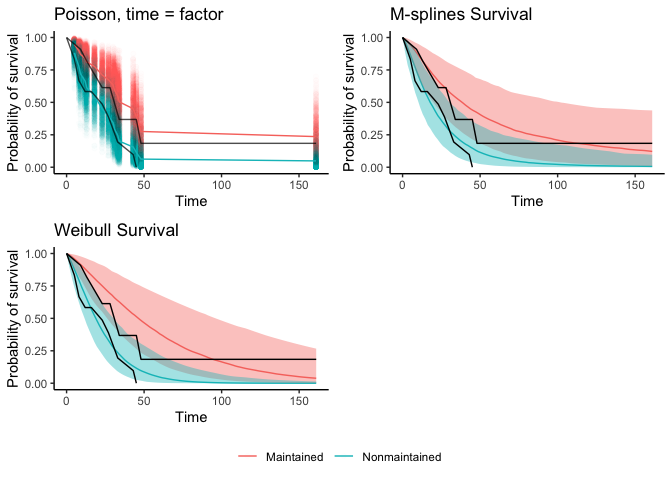

There you have it–3 different survival curves. (The poisson time as spline function produces a nice fitting survival curve too, but Rmarkdown is being buggy.) They all look like pretty good fits to the observed data (in black) and the weibull baseline function seems the worst. There are ways to make a smooth function of the upper left plot, but I didn’t feel like figuring it out. You can compare the models with loo, but beware that the function assumes each row of data is a new observation. It’s better aggregate the log-likehoods by subject so you leave one subject out instead of leaving one row out at a time.